

What is a Streaming SQL Engine?
A streaming SQL engine keeps queries’ results up to date without ever having to recalculate them, even as the underlying data changes. To explain this, imagine a simple query, such as <code-highlight>SELECT count(*) FROM humans<code-highlight> . A normal SQL engine (such as Postgres’s, MySQL’s) would need to go over all the different <code-highlight>humans<code-highlight> every time you ran that query- which could be quite costly and lengthy given our ever changing population count. With a streaming SQL engine, you would define that query once, and the engine would constantly keep the resulting count up to date as new humans were born and the old / sickly ones died off, without ever performing a recalculation of counting all humans in the world.
How to build a Streaming SQL engine
For the simple example above, you may have an idea of how a streaming SQL engine could work- first, you would need to do what any normal SQL engine does and calculate the number of humans. Next, every time a human was born you would add one to your result, and every time a human died you would negate one from your result. Easy, right?
Let’s try creating a diagram showing a procedural “query plan” and how we would process a new human being born. We’ll have a series of nodes, one for each operation, and a “final” node which will represent a table with our results. Since we’re a streaming engine and dealing with changes, we’ll represent the messages passed between our nodes as:

where the key is what we want to change, and the modification is by how much we want to change it. So for example, if we wanted to pass a message to a node telling it “Hey Mr. Node, 1.5 Apples have been added”, it would look like this:

Each node will be responsible for receiving changes, performing some type of operation, and then outputting changes itself. Another important concept here is that we can add modifications together if they have the same key. So the two changes <code-highlight>apple: 1.5<code-highlight> and <code-highlight>apple: 2<code-highlight> are equivalent to <code-highlight>apple: 3.5<code-highlight> . If the modifications equal zero together, it’s as if nothing at all happened- for example, if we have two changes <code-highlight>apple: 3<code-highlight> and <code-highlight>apple: -3<code-highlight> , it’s equivalent to not having streamed any changed (You can think of it as me giving you three apples, utterly regretting my kindness, then taking away your three apples. For you it would be as if nothing happened at all- aside from your broken pride). To make this make more sense, let’s draw out the nodes for our query (<code-highlight>SELECT count(*) FROM humans<code-highlight>), and add in the first human, Adam.
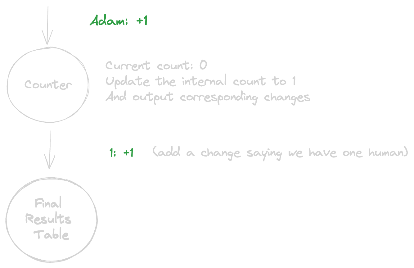
As we can see, a new human named “Adam” was born. The “Counter” node, perhaps called for its ability to count, holds an internal state of the current count of humans in the world. Whenever it receives a change (an addition or deletion of a human), it updates its internal count, and then outputs relevant changes- in this case, only one change was necessary, telling the next node to add the number one (signifying the total number of humans) once. In this instance, the next node was the “Final Results Table”, an actual honest-to-god relational table (perhaps in Postgres). You can imagine every change translating to a <code-highlight>DELETE<code-highlight> or <code-highlight>INSERT<code-highlight> based on the key and modification.
Next, let’s add in Eve:
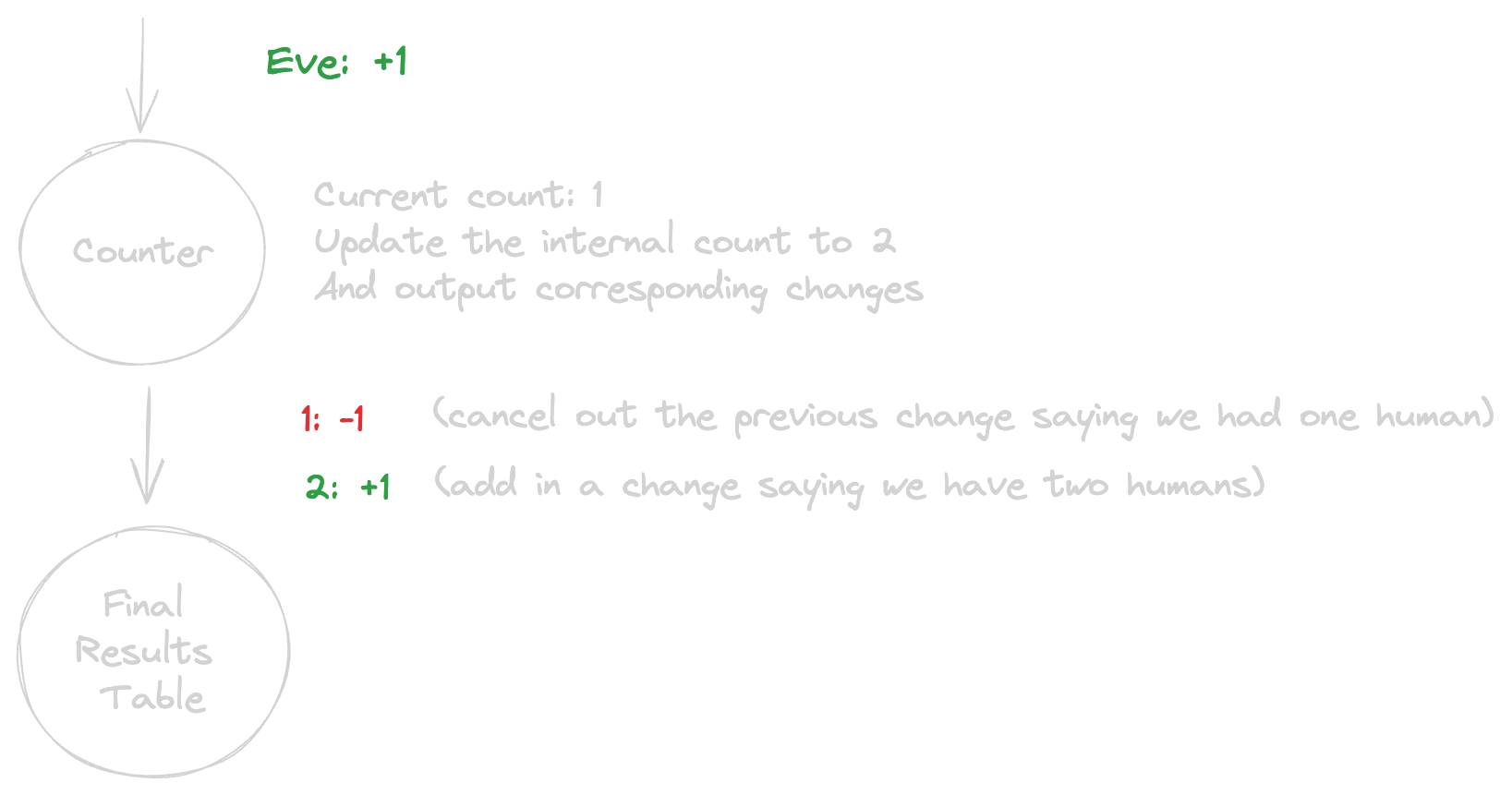
This time, the counter node needed to output two changes- one to cancel out the previous change it outputted, and one two add the new updated value. Essentially, if we were to look at all the changes the Counter node outputted over time, we’d get:
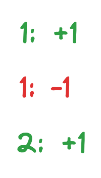
Since we’re allowed to combine changes with the same key, the above is equivalent to:
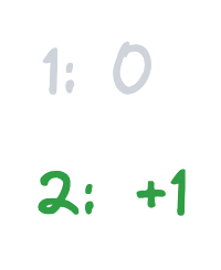
A modification of zero means we can simply remove the change. Therefore, we’re left only with <code-highlight>2: +1<code-highlight> in the final result table- exactly what we wanted.
Are you starting to feel that sweet sweet catharsis? Ya, me too.
A slightly more interesting example
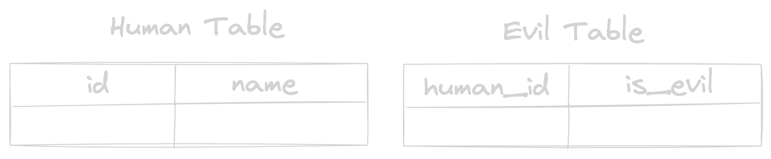
Let’s imagine we’re the devil and have two tables:
1. A “Human Table” that contains two columns, a unique identifier and their name.
2. An “Evil Table” that maps human ids to whether or not they are evil.
Now, for obvious reasons, let’s say we wanted a count of evil humans per name:
To be able to create a query plan (a series of nodes) from this query, we’re going to need to introduce a few new types of nodes here.
Filter Node
A filter node filters a change by its key, regardless of its modification. If a change “passes” the filter, the filter outputs it as is. To really give you the feel of this, let’s diagram a filter node that passes only changes with keys that are equal to the word “cats”.
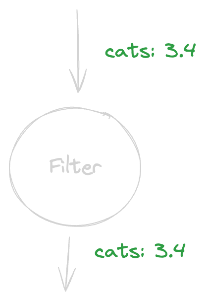
As we can see, we gave the filter node 3.4 cats and, astonishingly enough, it passed them on without changing a thing. Let’s try passing dogs through the filter node:
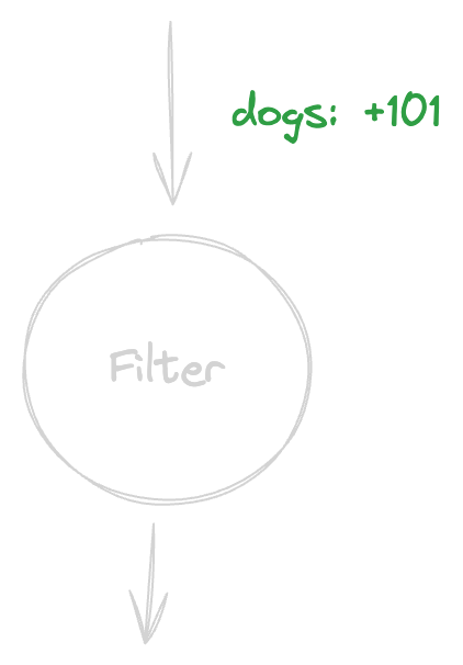
Whoa! This time the filter did not pass anything on. I imagine you get the idea. Moving on.
Joins
A Join node is responsible for receiving changes from two nodes, and outputting changes whose “join keys” match. It does this by holding an internal state (all in storage) of all the changes that pass through it from both sides, mapped by their respective join keys. So in our example with
we would create one Join node, with two mappings:
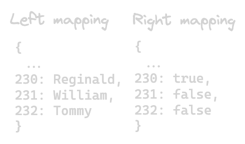
On the left side, for <code-highlight>id<code-highlight> to <code-highlight>name<code-highlight>
On the right side for <code-highlight>human_id<code-highlight> to <code-highlight>is_evil<code-highlight>
In practice, the mappings would look something like this:
Every time the Join node would receive a change from one of its sides, it would look on the other side for a matching key. If it found one, it would output the combined values. Let’s try drawing out a simple example where the Join node receives a new human named Tommy with id 232, and then a change saying id 232 is not evil.
First- a new human named Tommy enters the world:
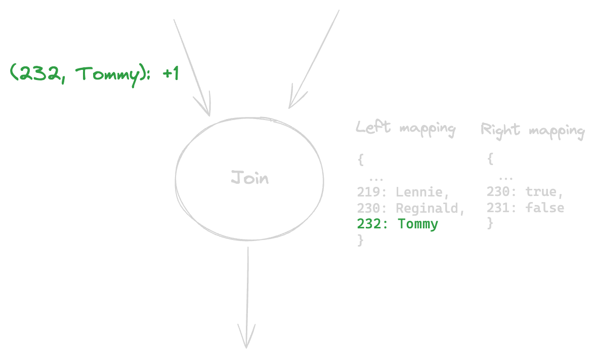
Ok, we streamed a change that tells the Join node that Tommy (id 232) has been added. The Join node looks in its right mapping for a corresponding change for key 232, and finds none. It therefore outputs nothing; but it does update its internal mapping to reflect the fact Tommy has been added- this will help us when we do the following:
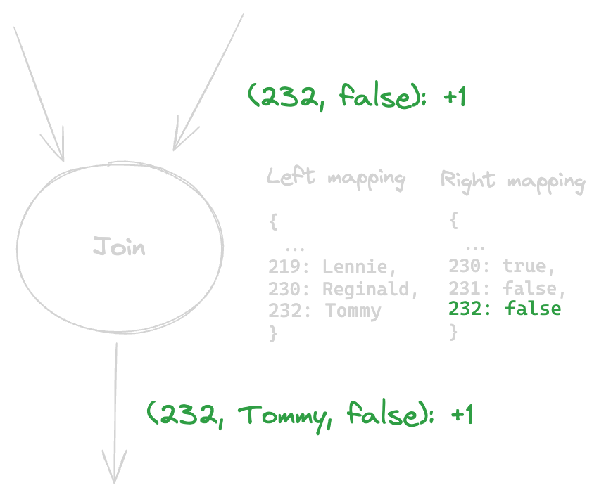
Here, the Join node received a change from its right side telling it “id 232 is not evil”. The Join node then looked at its left mappings, found a corresponding change (232: Tommy- the change we just streamed before) and outputted the combined change.
But this is not the end of the Tommy saga- at any moment new changes could come in. Perhaps Tommy could fall down the steps and die. This would result in the Join receiving <code-highlight>Tommy, 232: -1<code-highlight>, which would then have the Join node outputting <code-highlight>(232, Tommy, false): -1<code-highlight>— cancelling out the previous change the Join sent. Or perhaps Tommy could change in his evilness- we’ll keep that idea for an example down the line.
— -
Side note- you may have noticed we said “join key to change” but don’t actually keep the modification count in the join mapping. In the real world we do, and then multiply the modification counts of both sides to get the outputted modification count
— -
Group Bys
Our “Group By” node is very similar to the counter node we had before (in truth, they are one and the same wearing different hats- but that’s a tale for another time). The Group By node outputs aggregates per buckets- always ensuring that if you were to combine all changes it outputted, you would be left with at most one change per bucket (similar to how we took all the changes over time that came out of the Counter node, and saw that we’re left with only one as others cancel out). It does this by holding an internal mapping (in storage) between each bucket and its aggregated value. So in our example
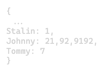
The Group By node would hold a mapping something like this:
Let’s try drawing out a simple example showing what would happen if we entered a new name the Group By node has never seen before:
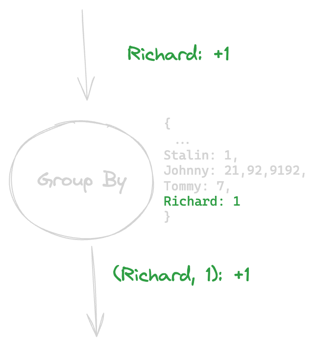
Ok, what happened here? The change coming into the Group By node tells the Group By node to add one to Richard. The Group By node looks in its internal mappings, and sees it has no entry for Richard. It adds an entry, and then outputs that the amount of Richards is one (this is the key of the change- <code-highlight>(Richard, 1)<code-highlight> ). Let’s go ahead and add another two Richards:
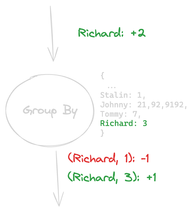
Slightly more interesting- the Group By node receives another change telling it to add two to Richard. The Group By node updates its internal state, and then outputs two changes- one to remove the previous change it outputted, and one to add a change with the new updated count of Richards.
Putting it all together
Back to our original query:
To set the stage for our upcoming example, imagine a young goody-two-shoes coder named Tommy, id 232 (you may remember him long ago from our explanation about the join). Tommy was a super cool dude who regularly downvoted mean people on StackOverflow (evilness=false).
One day, Tommy got kicked in the head by a horse, and as a direct result force pushed to master while deleting the CI. We’ll represent this occurrence with two changes- one to cancel out the old change saying Tommy wasn’t evil <code-highlight>(232, false): -1<code-highlight> , and one to add in the new change saying he is evil <code-highlight>(232, true): +1<code-highlight> :
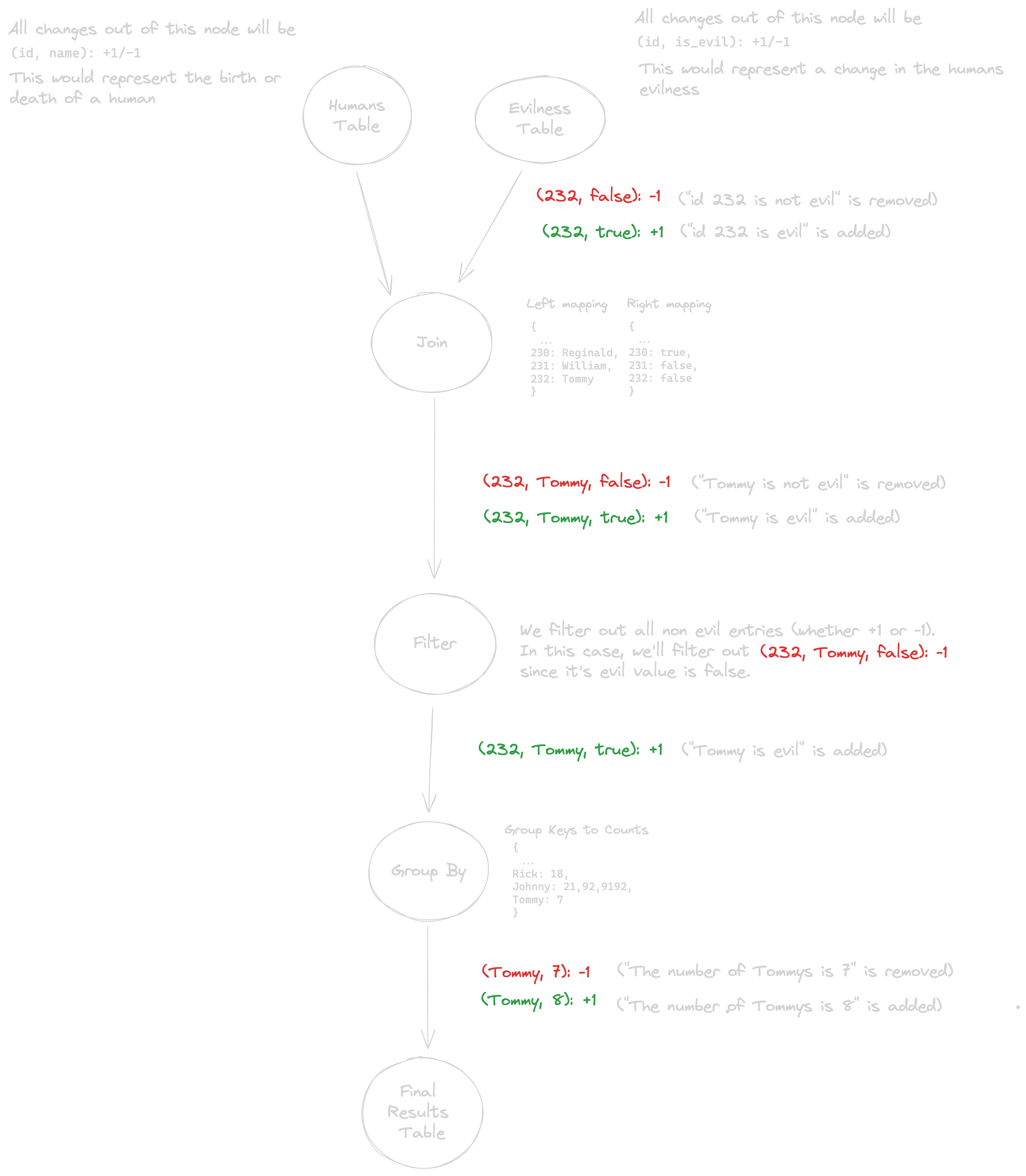
Let’s do a quick breakdown of what we see above- so we outputted the two changes we talked about <code-highlight>(232, false): -1<code-highlight> and <code-highlight>(232, true): +1<code-highlight> . The Join node receives it, looks on its other side (ids -> names), finds a name (Tommy), and outputs the inputted changes together with the name “Tommy”. Next, the filter node <code-highlight>WHERE is_evil IS true<code-highlight> filters out the change <code-highlight>(232, false): -1<code-highlight> , and, since its evil value is false, only outputs <code-highlight>(232, true): +1<code-highlight> . The Group By node takes in this change, looks in its mappings, and sees there existed a previous entry for Tommy (while not a very evil name, I have met some mean Tommys in my life). The Group By node therefore sends out one change to remove the old change it sent out with <code-highlight>(Tommy, 7): +1<code-highlight> (this happened in a previous addition of an evil Tommy). It then sends out another change introducing the new change to the Tommy count.
Wait, but why go to all the trouble?
So, now there are 8 Tommy’s in the world that are evil, and we didn’t need to rerun our query to calculate this. You may be thinking- well, Mr. Devil, you really didn’t need a streaming SQL engine to do that. If you had a humans table and evilness table, just create indexes on them. You’d still need to go over all the records each time queried, but at least the lookups would be quick. The Group By would still need to do everything from scratch, but at least…
So yes, it is possible to optimize queries so they run fairly quickly on the fly- up to a certain point. As more Joins, Group Bys, and (god forbid) WITH RECURSIVEs are added, it becomes more and more complex to optimize queries. And as more Tommys and Timmies and Edwards and Jennies (not to mention Ricardos and Samuels and Jeffries and Bennies) are added to our system, even those optimizations might begin to not be enough (and don’t even get me started on the evils of in-house caching). Streaming SQL engines are, to paraphrase a non-existent man, totally badass, and straight up solve this.
In Conclusion
Feel ready to build a streaming engine? You definitely have the building blocks- but you’re missing a few major concepts here such as how to be consistent (to never output partial results), how to do this all with high throughput (in everlasting tension with latency), and how to interact well with storage (async-io anyone?). Maybe I’ll write another blog post, maybe not.
By the way, as for the Lord dropping a table owned by another user: it apparently comes down to if he uses RDS (on a self-hosted DB he’s a superuser, but on RDS nobody is. Yes, not even the Lord).
Since posting this article, the Elders at Epsio realized there’s no point to keeping their secrets so secret and published their streaming engine for the world to use- check out Epsio’s blazingly fast SQL engine here.