PostgreSQL Bigger != Better

As part of our work at Epsio, we have the opportunity to speak with many companies trying to improve the performance of complex PostgreSQL queries running in their production systems.

Many times, we hear of companies trying to scale their instance sizes in an attempt to make their queries more performant. Usually, they expect that the bigger they make their instances, the faster their queries will run:

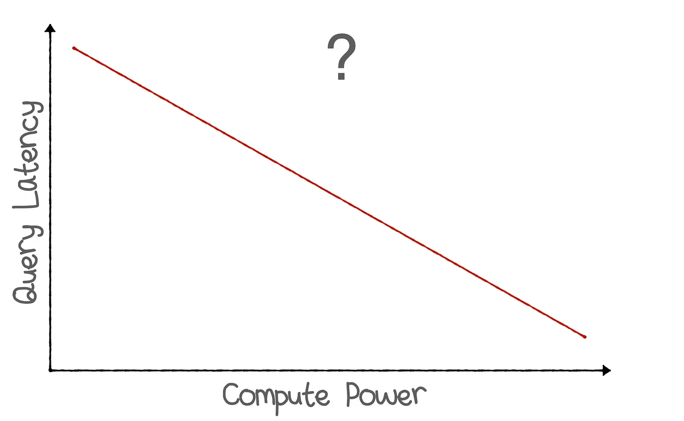
Although this is true many times, particularly for companies running many “simple” queries in parallel (such as retrieving a user’s past orders or fetching their email), companies with more “complex” backend queries (such as getting the 5 most purchased items in the entire system) usually find that increasing instance sizes doesn’t necessarily translate into better performance.

In this blog post, we will see how complex SQL queries scale as machine sizes increase, and try to learn where PostgreSQL doesn’t utilize its resources to their fullest potential when running analytical or complex queries :)

The Setup - TPC-H Queries

To simulate a good mix of complex queries, we used the TPC-H benchmark and ran it on various machine sizes running PostgreSQL 15 (on RDS M5 series).

The TPC-H benchmark consists of 22 queries, most of which involve many JOINs, ORDER BYs, and other operations that you would see in any other complex PostgreSQL query.


-- QUERY #3
SELECT
    l_orderkey,
    sum(l_extendedprice * (1 - l_discount)) as revenue,
    o_orderdate,
    o_shippriority
FROM
    CUSTOMER,
    ORDERS,
    LINEITEM
WHERE
    c_mktsegment = ':1'
    AND c_custkey = o_custkey
    AND l_orderkey = o_orderkey
    AND o_orderdate < date ':2'
    AND l_shipdate > date ':2'
GROUP BY
    l_orderkey,
    o_orderdate,
    o_shippriority
ORDER BY
    revenue desc,
    o_orderdate
LIMIT 10;

How did we measure Query Latency?

To ensure that our results are as accurate and as helpful as possible, we simulated a production deployment. We ran all 22 queries one after another from an EC2 machine located in the same region as the RDS machine.

After running the 22 queries, we calculated the geometric mean of query latency for that machine size. We used the geometric mean instead of a regular average because it treats a 50 percent performance boost the same for all queries, regardless of their latency. You can read more about the differences here.

Attempt #1 — Default RDS configuration

On our first attempt, we ran all 22 TCP-H queries with the default RDS configuration:

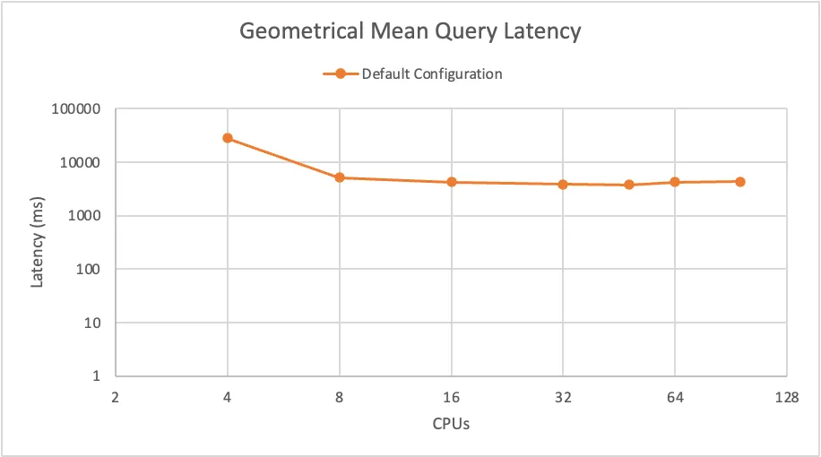
When examining the results, we could quickly see that although there was a performance boost going from 4 CPUs to 8 CPUs, there was barely any improvement increasing the machine size to more than 8 CPUs. Surprisingly, the performance even got worse going from 48 CPUs to 64 CPUs.

Since the vast majority of companies we work with already have a production deployment of more than 8 CPUs, this unfortunately means that the idea of “more compute, faster queries” does not seem to hold true with the default PostgreSQL configuration.

To try to “explain” and “analyze” this, we did what any other developer would do in this situation: we ran EXPLAIN ANALYZE (a PostgreSQL command that displays statistics and information about a query you run) on the 32 CPUs machine:


--- TPC-H Query running on 32 CPUs machine
tpch=> EXPLAIN ANALYZE select c_name, c_custkey, o_orderkey, o_orderdate, o_totalprice, sum(l_quantity) from customer, orders, lineitem w ......
...
        ->  Gather Merge  (cost=3472688.11..3555768.51 rows=712068 width=38) (actual time=49382.693..55001.291 rows=15015381 loops=1)
              Workers Planned: 2
              Workers Launched: 2
              ->  Sort  (cost=3471688.09..3472578.17 rows=356034 width=38) (actual time=47629.540..49850.869 rows=5005127 loops=3)
                    Sort Key: lineitem_1.l_orderkey
...

Even though our machine had 32 CPUs, PostgreSQL has chosen to launch only 2 workers (which means it used only 2 CPUs) to execute the query, utilizing only 1/16th of the available computing power! Not cool, Postgres! Just kidding, we love you.

After a quick online search (thanks pgmustard for a great blog post about configurations for parallel queries!), we discovered that this probably happened because PostgreSQL (and RDS) has a default configuration value of max_parallel_workers_per_gather set to 2.

Takeaway: Queries running on the default RDS/PostgreSQL configuration will only use up to 2 CPUs!

Attempt #2 — max_workers_per_gather=100

As the next step, we changed this parameter’s value to 100 and re-ran the benchmark to see how the change would affect our results:

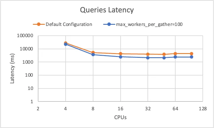
Even though the results improved, they definitely didn’t improve as we expected them to. Instead of “more compute, faster queries”, it was still “more compute, kind of the same performance”.

To try explaining and analyzing this (yes, I used the same joke twice), we ran EXPLAIN ANALYZE, and were surprised to discover that PostgreSQL had still not fully utilized it’s resources and used only 7 workers for our complex query:


tpch=> EXPLAIN ANALYZE select c_name, c_custkey, o_orderkey, o_orderdate, o_totalprice, sum(l_quantity) from customer, orders, lineitem w ……
...
       -> Gather Merge (cost=2095052.72..2399297.50 rows=2476411 width=38) (actual time=11118.089..14990.743 rows=15016549 loops=1)
           Workers Planned: 7
           Workers Launched: 7
           ->  Sort  (cost=2094052.60..2094937.04 rows=353773 width=38) (actual time=10412.230..10897.991 rows=1877069 loops=8) Sort Key: lineitem_1.l_orderkey
...

Although we had additional configurations we could tinker with to “politely” ask PostgreSQL to make more use of its resources, we are not known to be “polite” people and decided to get dirty and use an “unconventional weapon”.

Attempt #3 — SET (parallel_workers = …)

To try to force PostgreSQL to use all its CPUs for our queries (with the hope that it will make them faster), we decided that a good next step would be to use [.code]ALTER TABLE table_name SET (parallel_workers=…);[.code] This configuration forces PostgreSQL to use as many parallel workers as you tell it to when accessing a table.

Obviously, this configuration is not recommended for production deployments as it forces PostgreSQL to spin up many workers even for the simplest operation on that table, leading to significant resources being consumed for every simple operation.

We configured parallel_workers to match the number of CPUs on each machine had, ran the benchmark, and……..

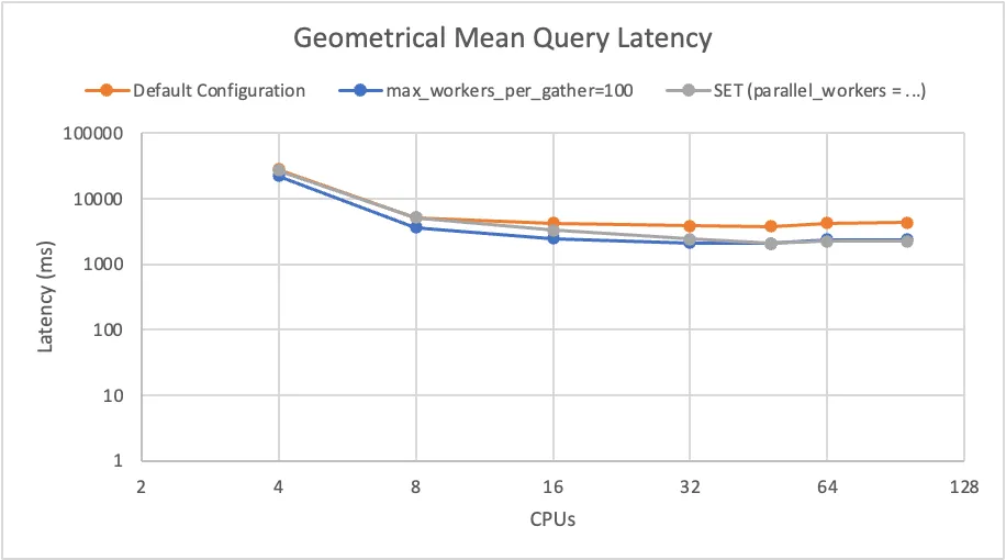
Funnily enough — this configuration seemed to not only not help, but also to increase the latency on the 16 CPUs machine.

So — why don’t queries get faster with more resources?

For those of you who are expecting to soon find the reason we discovered why PostgreSQL didn’t scale well, I wouldn’t get your hopes up. After analyzing the query plan of all 22 TPC-H queries, reading online about the subject, and asking people we trust in the field, it seems that there is not just one big reason why PostgreSQL can’t parallelize these queries efficiently. Looking back, this makes a lot of sense since if there were only one reason, the PostgreSQL community would probably just fix it.

Scaling and parallelizing queries properly is no easy task for a database, especially for one primarily built for a completely different use case (simple transactional queries). Although PostgreSQL has made amazing progress in recent years supporting workloads like the one we tested (until 2016, PostgreSQL didn’t have parallel query execution at all), there still seem to be many small and incremental changes that will need to occur before PostgreSQL can properly scale these workloads.

Having said this, while looking at the TPC-H queries, we have still noticed a couple of specific scenarios where there was an “obvious” reason why PostgreSQL did not get faster with more resources. You might want to know these scenarios so that you can avoid them in the future when trying to optimize a query.

#1 — CTEs & Sub-Queries can sometimes cause only a part of the query to run in parallel

Although it is not always the case (depending on the specific logic written in them), many times CTEs, scalar subqueries, or even normal subqueries will not run the outer part of the query in parallel.

While in this scenarios, a large part of the query can still run in parallel, there is a certain limit to how much a query can be optimized given there is always a part of it the won’t run in parallel (see Amdahl’s law).

For example, you can see in this TPC-H query that the PostgreSQL used 16 workers for the initial Gather, but then ran a hash join on top of the gathered result with a single worker (i.e., process):


--------------------------------------------------------------------------------------------------------------------------------------------------------------------------
 Aggregate  (cost=2132667.85..2132667.86 rows=1 width=32) (actual time=17591.529..17591.714 rows=1 loops=1)
   ->  Hash Join  (cost=45036.00..2132616.07 rows=20712 width=8) (actual time=27.975..17590.323 rows=5156 loops=1)
         Hash Cond: (lineitem.l_partkey = part.p_partkey)
         Join Filter: (lineitem.l_quantity < (SubPlan 1))
         Rows Removed by Join Filter: 53561
         ->  Seq Scan on lineitem  (cost=0.00..1928815.84 rows=60004684 width=19) (actual time=0.007..4524.988 rows=60005970 loops=1)
         ->  Hash  (cost=45010.11..45010.11 rows=2071 width=6) (actual time=22.526..22.710 rows=1970 loops=1)
               Buckets: 4096  Batches: 1  Memory Usage: 108kB
               ->  Gather  (cost=1000.00..45010.11 rows=2071 width=6) (actual time=0.760..22.411 rows=1970 loops=1)
                     Workers Planned: 16
                     Workers Launched: 16
                     ->  Parallel Seq Scan on part  (cost=0.00..43803.01 rows=129 width=6) (actual time=0.186..16.542 rows=116 loops=17)
                           Filter: ((p_brand = 'Brand#52'::bpchar) AND (p_container = 'JUMBO PACK'::bpchar))
                           Rows Removed by Filter: 117531
         SubPlan 1
           ->  Aggregate  (cost=125.17..125.18 rows=1 width=32) (actual time=0.037..0.037 rows=1 loops=58717)
                 ->  Index Scan using lineitem_part_supp_fkidx on lineitem lineitem_1  (cost=0.56..125.09 rows=30 width=5) (actual time=0.009..0.032 rows=31 loops=58717)
                       Index Cond: (l_partkey = part.p_partkey)
 Planning Time: 0.321 ms
 Execution Time: 17591.755 ms
(20 rows)

#2 — Some operators won’t run in parallel at all

Some operators in PostgreSQL cannot run in parallel. If you use these operators, your entire query / gather operation will run on a single worker. These operators include:

Additionally, some operators / query plans can run in parallel but are less efficient in that mode, meaning PostgreSQL might choose to run the query in a single process even though it can parallelize it. For example, Joins that are using a merge join, can scan the outer set in parallel, but must scan the inner set repeatedly in every worker (as seen in this article). This means that launching 32 workers will result in scanning the full outer set 32 times (which is not very cost-effective). Therefore, the planner might choose not to parallelize it, even though it can.

TPC-H Query #13, for example, was never parallelized in our workload because it used merge join (even with the configuration forcing it to use parallel_workers):


tpch=> EXPLAIN ANALYZE select c_count, count(*) as custdist from ( select c_custkey, count(o_orderkey) as c_count from customer left outer join orders on c_custkey = o_custkey and o_comment not like '%express%packages%' group by c_custkey) c_orders group by c_count order by custdist desc, c_count desc;
                                                                                  QUERY PLAN                                                                                  
------------------------------------------------------------------------------------------------------------------------------------------------------------------------------
 Sort  (cost=1883122.42..1883122.92 rows=200 width=16) (actual time=19925.969..19925.973 rows=46 loops=1)
   Sort Key: (count(*)) DESC, (count(orders.o_orderkey)) DESC
   Sort Method: quicksort  Memory: 27kB
   ->  HashAggregate  (cost=1883112.78..1883114.78 rows=200 width=16) (actual time=19925.948..19925.956 rows=46 loops=1)
         Group Key: count(orders.o_orderkey)
         Batches: 1  Memory Usage: 40kB
         ->  GroupAggregate  (cost=61.47..1860612.86 rows=1499995 width=14) (actual time=0.044..19685.781 rows=1500000 loops=1)
               Group Key: customer.c_custkey
               ->  Merge Left Join  (cost=61.47..1770629.27 rows=14996728 width=12) (actual time=0.022..17324.743 rows=15287777 loops=1)
                     Merge Cond: (customer.c_custkey = orders.o_custkey)
                     ->  Index Only Scan using customer_pk on customer  (cost=0.43..38964.35 rows=1499995 width=6) (actual time=0.010..153.560 rows=1500000 loops=1)
                           Heap Fetches: 0
                     ->  Index Scan using order_customer_fkidx on orders  (cost=0.43..1540455.83 rows=14996728 width=12) (actual time=0.009..14122.213 rows=14787771 loops=1)
                           Filter: ((o_comment)::text !~~ '%express%packages%'::text)
                           Rows Removed by Filter: 212229
 Planning Time: 0.303 ms
 Execution Time: 19926.018 ms
(17 rows)

About Epsio

Epsio is an incremental engine that plugs into existing databases and constantly updates results of complex queries you define whenever the underlying data changes, without ever needing to recalculate the entire dataset. This means Epsio can provide instant and up-to-date results for complex queries (while also reducing compute costs!).